[EN] Basic example of use - gridmarthe 101
The gridmarthe package is designed to facilitate reading/writing grids in the Marthe format. This notebook allows you to explore some basic features of the package and shows an example of grid processing.
# import package
import gridmarthe as gm
gridmarthe library is based on xarray, which enhances working with multidimensional grids.
Full documentation is available at:
https://docs.xarray.dev/en/stable/index.html
Basic features
Marthe Grids contain metadata, including the time step index, but not the actual dates. Therefore, it is useful to provide the reading function either with a series of dates (to be constructed manually) or a timestep file so that the dates are read automatically.
Additionally, several arguments can be useful for reading (removal of null values, transformation of xy, addition of mesh indicator or column/row numbers, etc.).
To check for possible options, you can display the function’s help.
help(gm.load_marthe_grid)
Help on function load_marthe_grid in module gridmarthe.grid.io.gridmarthe:

load_marthe_grid(filename: str, varname: Optional[str] = None, fpastp: Optional[str] = None, dates=None, drop_nan: bool = False, nan_value: Union[int, float, list, NoneType] = None, xyfactor: Union[int, float] = 1.0, shallow_only=False, add_col_row: bool = False, add_id_grid: bool = False, title: Optional[str] = None, var_attrs: dict = {}, epsg: int = 27572, full_3d: bool = False, drop_time: bool = False, model_attrs: dict = {'domain': 'FR-France', 'institution': 'BRGM, French Geological Survey, Orléans, France'}, engine: str = 'xarray', verbose: bool = False, **kwargs)
    Read Marthe Grid File as xarray.Dataset

    The gridfile is read as a sequence: the variable for all layer
    for main grid, then all layer for nested grids, is stored in
    a 1D vector for every timestep. A single spatial identifier
    ``zone`` is used to map spatial coordinates.

    Before plot operations, user can assign coordinates (set x,y
    as dimension coordinates and drop zone) to get 2-D arrays (or
    3D arrays if multilayer) for every timesteps.

    Note
    ----

    A former known issue with some version of Marthe is that field name is
    not written in metadata, as number of nested grids or number of layers., which
    This can cause some bug when reading grids with gridmarthe.
    As of `gridmarthe` version 0.4, if no varname is scanned in file and/or number of layer/grids
    are missing, these informations are guessed when parsing data, which are stored in
    a variable named 'variable' and a warning is raised to alert user to rename the
    variable later. This is only valid for parameters grids (with only one timestep).
    In case of remaining errors, the command line tool `cleanmgrid`
    (provided with gridmarthe) can still be used to clean the file and add missing metadata.

    Parameters
    ----------
    filename: str
        A path to marthegrid file (.permh, .out, etc.)

    varname : str, optional
        Variable to access in martgrid file. See marthegrid (`filename`) file content.

        - If None  is passed (default), function will scan all varnames in filename
        and keep first only.

        - If a varname is passed, e.g ``CHARGE`` for groundwater head, the returned
        dataset will contains only this variable.

        - If 'all' is passed,  function will scan all varnames in filename and keep all.
        All datavars are added to dataset, using recursive call to func

        - If wrong variable name is passed, empty data will be returned.

    fpastp: str, optional
        A pastp file to read for dates

    dates: sequence, optional
        Can be a pd.date_range, pd.Series, pd.DatetimeIndex, np.array or list of
        datetime/np.datetime objects.
        If no dates (or no fpastp) is provided, a fake sequence of dates from
        1850 to 1900 will be used for xarray object

    drop_nan: bool, optional
        Drop nan values (corresponding to nan_value) in xarray object to return.
        Default is False (keep nan values).

    nan_value: float or list of float, optional
        A code value for nan values. The default value is inferred from field name.
        E.g. of default nan values:

        - hydraulic conductivity: 0 or -9999. (Warning: a value of +9999. is not
          a NaN value for hydraulic conductivity. See Marthe User Guide for explanation
          about this code, refering here to impervious layer);

        - hydraulic head: 9999.;

        - groundwater flow: 0. (9999. is used as special value for this field);

        - any other: 9999.

    xyfactor: int or float, optional
        factor to transform X and Y values. e.g.: 1000 to convert km XY to meters.
        Default is 1.

    shallow_only: bool, optional
        Boolean to read only the first layer. Default is False.
        Warning: only valid for NON nested grids for now.

    add_col_row: bool, optional
        Add columns (col) and rows (row, formerly lig (v<=0.1.3)) index (from 1 to n).
        Default is False.

    add_id_grid: bool, optional
        Add grid id (from 0 to n), useful for nested grids.
        0 is main grid, Default is False

    title: str , optional
        Title for grid attributes. Default is None (not used)

    var_attrs: dict, optional
        Dictionnary of attributes to add to variable DataArray.

    epsg: int, optional
        EPSG code for projection. Default is 27572 for legacy reasons (Lambert 2 Etendu,
        for France). Used to write CRS information in attributes. Useful for GUI
        (eg visualisation in QGIS).

    full_3d: bool, optional
        Is z dimension an aquifer layer or real Z axis (in meters for exemple)
        Default is False (z is aquifer layer number)

    drop_time: bool, optional
        Drop time dimension even if only one timestep is present.
        Default is False. If True and only one timestep, time dimension is removed.
        Useful for parameters grids.

    model_attrs: dict, optional
        Dictionnary of attributes to add to Dataset.
        by default, gis attrs are added and can be modified

        >>> {
        ...    'domain': 'FR-France',
        ...    'institution': 'BRGM, French Geological Survey, Orléans, France'
        ... }

        For example, if your data is associated with a reference (report, paper, etc.):

        >>> {
        ...    'references': 'https://doi.org/...'
        ... }

    engine: str, optional
        Engine to use for returned object. Default is 'xarray', which return
        xarray.Dataset object.
        Another option is 'numpy', which return a list of numpy arrays :
        [zvar, zdates, isteps, zxcol, zylig, zdxlu, zdylu, ztitle, dims]

    verbose: bool, optional
        Print some information about execution in stdout.
        Default is False.

    Returns
    -------
    ds: xr.Dataset
        A xarray.Dataset object containing values and attributes read from Marthe
        grid file.
# reading data and storing into Dataset object (with xarray)
ds = gm.load_marthe_grid(
    './data/chasim_hallue.out', 'CHARGE',
    fpastp='./data/hallue.pastp',
    drop_nan=True
)
# display values and attributes
display(ds)
<xarray.Dataset> Size: 2MB
Dimensions:  (time: 205, zone: 927)
Coordinates:
  * time     (time) datetime64[ns] 2kB 1995-07-31 1995-08-01 ... 2012-07-01
  * zone     (zone) int32 4kB 255 256 257 258 259 ... 2722 2723 2724 2725 2726
Data variables:
    charge   (time, zone) float64 2MB 100.0 100.6 101.1 ... 27.0 26.0 26.35
    x        (zone) float32 4kB 617.8 618.2 618.8 619.2 ... 606.8 607.2 607.8
    y        (zone) float32 4kB 2.567e+03 2.567e+03 ... 2.543e+03 2.543e+03
    dx       (zone) float32 4kB 0.5 0.5 0.5 0.5 0.5 0.5 ... 0.5 0.5 0.5 0.5 0.5
    dy       (zone) float32 4kB 0.5 0.5 0.5 0.5 0.5 0.5 ... 0.5 0.5 0.5 0.5 0.5
    izone    (zone) int32 4kB 1 2 3 4 5 6 7 8 ... 921 922 923 924 925 926 927
Attributes: (12/17)
    conventions:          CF-1.10
    title:                Modélisation du bassin de la SOMME Nappe_Libre
    marthe_grid_version:  9.0
    original_dimensions:  x,y,z [grids]: 53 54 1
    crs:                  {'crs_wkt': 'PROJCRS["NTF (Paris) / Lambert zone II...
    lon_resolution:       0.5
    ...                   ...
    period:               1995-2012
    frequency:            30 day(s)
    creation_date:        Created on 2026-07-10T18:00:51Z UTC
    comment:              Hydrogeological model created with MARTHE code (Thi...
    domain:               FR-France
institution: BRGM, French Geological Survey, Orléans, FranceThe grid is loaded into a 2D xarray object (reduced horizontal grid), with dimensions (time, zone).
The spatial dimension is thus 1D, contained in zone. Each zone has a pair of xy coordinates, stored as a variable (not as a dimension).
This format allows many operations to be performed more efficiently than in 2 or 3D + time.
You just need to assign the coordinates (transform to 2 or 3D + time) before using graphical features.
# add coordinates to transform the 2D Dataset into 3D
ds_3d = gm.assign_coords(ds)
display(ds_3d)  # check new coordinates
<xarray.Dataset> Size: 3MB
Dimensions:  (y: 48, x: 44, time: 205)
Coordinates:
  * y        (y) float32 192B 2.567e+03 2.566e+03 ... 2.544e+03 2.543e+03
  * x        (x) float32 176B 599.2 599.8 600.2 600.8 ... 619.8 620.2 620.8
  * time     (time) datetime64[ns] 2kB 1995-07-31 1995-08-01 ... 2012-07-01
Data variables:
    charge   (time, y, x) float64 3MB nan nan nan nan nan ... nan nan nan nan
    dx       (y, x) float32 8kB nan nan nan nan nan nan ... nan nan nan nan nan
    dy       (y, x) float32 8kB nan nan nan nan nan nan ... nan nan nan nan nan
    izone    (y, x) float64 17kB nan nan nan nan nan nan ... nan nan nan nan nan
Attributes: (12/17)
    conventions:          CF-1.10
    title:                Modélisation du bassin de la SOMME Nappe_Libre
    marthe_grid_version:  9.0
    original_dimensions:  x,y,z [grids]: 53 54 1
    crs:                  {'crs_wkt': 'PROJCRS["NTF (Paris) / Lambert zone II...
    lon_resolution:       0.5
    ...                   ...
    period:               1995-2012
    frequency:            30 day(s)
    creation_date:        Created on 2026-07-10T18:00:51Z UTC
    comment:              Hydrogeological model created with MARTHE code (Thi...
    domain:               FR-France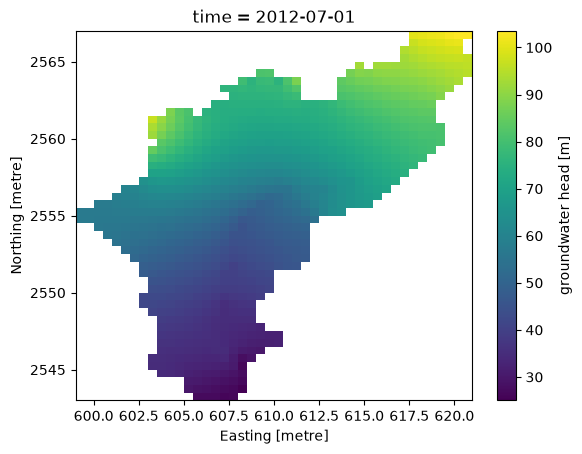
institution: BRGM, French Geological Survey, Orléans, France# plot for a given time step
ds_3d.isel(time=-1)['charge'].plot.pcolormesh()
<matplotlib.collections.QuadMesh at 0x7e379ff329f0>
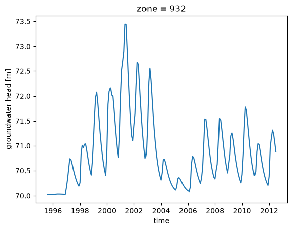
# or plot for a given zone (over time)
ds.isel(zone=255)['charge'].plot()
[<matplotlib.lines.Line2D at 0x7e379f85a630>]
For nested grids, a specific plotting function is provided (gm.plot_nested_grids()).
For models with multiple layers, you can retrieve the surface layers: gm.get_min_layer(ds, [subset_layers=[3,5]])
or even display this result: gm.plot_outcrop()
The native functions of xarray and numpy already allow grid modifications (value substitution, transformation, operations between two grids, etc.)
Advanced features
Handle computation over grids, with xarray and gridmarthe
# compute diff between grids
ds0 = ds.sel(time='1995-11-01')
ds1 = ds.sel(time='2001-02-01')

ds0['charge'] - ds1['charge']
<xarray.DataArray 'charge' (zone: 927)> Size: 7kB
array([ 0.00000e+00,  0.00000e+00,  0.00000e+00,  0.00000e+00,
        0.00000e+00,  0.00000e+00,  0.00000e+00,  0.00000e+00,
       -3.25440e-01, -4.60980e-01, -5.27480e-01, -5.59100e-01,
       -5.74500e-01,  0.00000e+00, -3.74970e-01, -6.81720e-01,
       -8.68420e-01, -9.77570e-01, -1.04721e+00, -1.09548e+00,
        0.00000e+00, -6.41230e-01, -1.00733e+00, -1.22240e+00,
       -1.35717e+00, -1.45930e+00, -1.57370e+00, -1.80513e+00,
        0.00000e+00,  0.00000e+00,  0.00000e+00,  0.00000e+00,
       -5.66100e-01, -1.02068e+00, -1.33316e+00, -1.53087e+00,
       -1.65762e+00, -1.74995e+00, -1.82523e+00, -1.90350e+00,
        0.00000e+00,  0.00000e+00, -1.43024e+00, -1.00962e+00,
       -1.14766e+00, -8.35060e-01, -7.87260e-01, -8.78120e-01,
       -1.16742e+00, -1.45697e+00, -1.68467e+00, -1.83483e+00,
       -1.92341e+00, -1.97372e+00, -1.99069e+00, -1.98500e+00,
        0.00000e+00,  0.00000e+00, -3.44370e-01, -3.57610e-01,
        0.00000e+00,  0.00000e+00,  0.00000e+00, -2.09688e+00,
       -1.83277e+00, -1.61107e+00, -1.55613e+00, -1.44464e+00,
       -1.43203e+00, -1.52037e+00, -1.68965e+00, -1.87151e+00,
       -2.02142e+00, -2.11349e+00, -2.14897e+00, -2.14145e+00,
       -2.09989e+00, -1.43919e+00, -1.36450e+00, -9.45770e-01,
...
       -6.78740e-01, -1.82235e+00, -1.73151e+00, -1.55717e+00,
       -1.30703e+00, -9.77720e-01, -5.57570e-01, -4.35400e-02,
       -1.44860e-01, -2.52990e-01, -3.26250e-01, -3.69900e-01,
       -4.01230e-01, -5.87460e-01, -6.72990e-01, -1.76108e+00,
       -1.67109e+00, -1.50200e+00, -1.26479e+00, -9.60430e-01,
       -5.85770e-01, -1.32270e-01, -3.03400e-02, -1.52940e-01,
       -1.90000e-01, -1.65750e-01,  0.00000e+00, -1.76839e+00,
       -1.72637e+00, -1.62543e+00, -1.45758e+00, -1.23024e+00,
       -9.55270e-01, -6.37120e-01, -3.04530e-01, -2.48100e-02,
       -7.04900e-02,  0.00000e+00,  0.00000e+00, -1.75184e+00,
       -1.68804e+00, -1.58243e+00, -1.41312e+00, -1.18093e+00,
       -9.31090e-01, -6.64310e-01, -3.79320e-01, -4.50800e-02,
       -1.84200e-02, -1.20000e-02, -1.64234e+00, -1.54945e+00,
       -1.37045e+00, -1.08295e+00, -8.56250e-01, -6.43070e-01,
       -4.37550e-01, -2.51870e-01, -1.76770e-01, -1.46430e-01,
       -8.46730e-01, -6.94620e-01, -5.40770e-01, -4.04770e-01,
       -2.89830e-01, -2.15860e-01, -1.52910e-01, -6.92440e-01,
       -4.57850e-01, -3.42300e-01, -2.65000e-01, -2.01410e-01,
       -1.59930e-01,  3.00000e-05,  0.00000e+00,  0.00000e+00,
       -2.06900e-02,  0.00000e+00, -1.24820e-01])
Coordinates:
  * zone     (zone) int32 4kB 255 256 257 258 259 ... 2722 2723 2724 2725 2726
Attributes:
    varname:             CHARGE
    units:               m
    mart_missing_value:  9999.0
    standard_name:       water_table_level
long_name: groundwater head# compute quantile
ds_5perc = ds.copy()
ds_5perc['q5'] = ds_5perc['charge'].quantile(0.05, dim='time')
ds_5perc['tresh'] = ds_5perc['charge'] < ds_5perc['q5']
ds_5perc
<xarray.Dataset> Size: 2MB
Dimensions:   (time: 205, zone: 927)
Coordinates:
  * time      (time) datetime64[ns] 2kB 1995-07-31 1995-08-01 ... 2012-07-01
  * zone      (zone) int32 4kB 255 256 257 258 259 ... 2722 2723 2724 2725 2726
    quantile  float64 8B 0.05
Data variables:
    charge    (time, zone) float64 2MB 100.0 100.6 101.1 ... 27.0 26.0 26.35
    x         (zone) float32 4kB 617.8 618.2 618.8 619.2 ... 606.8 607.2 607.8
    y         (zone) float32 4kB 2.567e+03 2.567e+03 ... 2.543e+03 2.543e+03
    dx        (zone) float32 4kB 0.5 0.5 0.5 0.5 0.5 0.5 ... 0.5 0.5 0.5 0.5 0.5
    dy        (zone) float32 4kB 0.5 0.5 0.5 0.5 0.5 0.5 ... 0.5 0.5 0.5 0.5 0.5
    izone     (zone) int32 4kB 1 2 3 4 5 6 7 8 ... 921 922 923 924 925 926 927
    q5        (zone) float64 7kB 100.0 100.6 101.1 101.6 ... 26.98 26.0 26.31
    tresh     (time, zone) bool 190kB False False False ... False False False
Attributes: (12/17)
    conventions:          CF-1.10
    title:                Modélisation du bassin de la SOMME Nappe_Libre
    marthe_grid_version:  9.0
    original_dimensions:  x,y,z [grids]: 53 54 1
    crs:                  {'crs_wkt': 'PROJCRS["NTF (Paris) / Lambert zone II...
    lon_resolution:       0.5
    ...                   ...
    period:               1995-2012
    frequency:            30 day(s)
    creation_date:        Created on 2026-07-10T18:00:51Z UTC
    comment:              Hydrogeological model created with MARTHE code (Thi...
    domain:               FR-France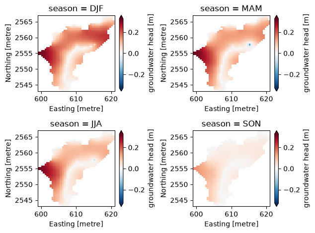
institution: BRGM, French Geological Survey, Orléans, France# compute anomaly
anom = ds.groupby("time.month") - ds.groupby("time.month").median(dim="time")
# rename new variable
ds_anom = ds.copy()
ds_anom['anom'] = anom['charge']
# compute seasonal mean
# 1st: mean head over each season...
ds_season = ds_anom.resample(time="QS-DEC").median(dim='time') # or .agg({"time": 'mean'})
# ... then aggregate all seasons
ds_season_agg = ds_season.groupby("time.season").mean(dim="time")
ds_season_agg  # mind the new dimension 'season'
<xarray.Dataset> Size: 152kB
Dimensions:  (season: 4, zone: 927)
Coordinates:
  * season   (season) object 32B 'DJF' 'JJA' 'MAM' 'SON'
  * zone     (zone) int32 4kB 255 256 257 258 259 ... 2722 2723 2724 2725 2726
Data variables:
    charge   (season, zone) float64 30kB 100.0 100.6 101.1 ... 26.99 26.0 26.33
    x        (season, zone) float32 15kB 617.8 618.2 618.8 ... 606.8 607.2 607.8
    y        (season, zone) float32 15kB 2.567e+03 2.567e+03 ... 2.543e+03
    dx       (season, zone) float32 15kB 0.5 0.5 0.5 0.5 0.5 ... 0.5 0.5 0.5 0.5
    dy       (season, zone) float32 15kB 0.5 0.5 0.5 0.5 0.5 ... 0.5 0.5 0.5 0.5
    izone    (season, zone) float64 30kB 1.0 2.0 3.0 4.0 ... 925.0 926.0 927.0
    anom     (season, zone) float64 30kB 0.0 0.0 0.0 ... -0.002924 0.0 0.001059
Attributes: (12/17)
    conventions:          CF-1.10
    title:                Modélisation du bassin de la SOMME Nappe_Libre
    marthe_grid_version:  9.0
    original_dimensions:  x,y,z [grids]: 53 54 1
    crs:                  {'crs_wkt': 'PROJCRS["NTF (Paris) / Lambert zone II...
    lon_resolution:       0.5
    ...                   ...
    period:               1995-2012
    frequency:            30 day(s)
    creation_date:        Created on 2026-07-10T18:00:51Z UTC
    comment:              Hydrogeological model created with MARTHE code (Thi...
    domain:               FR-France
institution: BRGM, French Geological Survey, Orléans, France# set coords for plot
ds_season_agg.update({
v: ds_season_agg[v].isel(season=0) # remove season dim for coordinates, appears in computation
for v in ['x', 'y', 'dx', 'dy']
})
ds_season_agg_2d = gm.assign_coords(ds_season_agg)
# Seasonal plot
import numpy as np
from matplotlib import pyplot as plt, colors

var = 'anom'
minval, maxval = ds_season_agg_2d[var].min(skipna=True).values, ds_season_agg_2d[var].max(skipna=True).values
fig, axes = plt.subplots(nrows=2, ncols=2)
axes = axes.ravel()
for i, season in enumerate(("DJF", "MAM", "JJA", "SON")):
    ds_season_agg_2d[var].sel(season=season).plot.pcolormesh(
            # x="x", y="lat",
            ax=axes[i],
            # cmap="Spectral",
            # vmin=minval, vmax=maxval,
            norm=colors.CenteredNorm(halfrange=np.max(np.abs([minval, maxval]))),
            add_colorbar=True,
            extend="both",
        )
plt.tight_layout()