[FR] Exemple d’utilisation de gridmarthe
Le package gridmarthe est conçu pour faciliter la lecture/l’écriture de grille au format Marthe. Ce notebook permet d’explorer quelques fonctionnalités de base du package et de montrer un exemple de traitement des grilles.
# import du package
import gridmarthe as gm
La librairie gridmarthe s’appuie sur xarray, qui permet de faciliter le traitement de grilles spatio-temporelles. La documentation complète de cette librairie est accessible :
https://docs.xarray.dev/en/stable/index.html
Fonctionnalités de base
Les grilles contiennent certaines métadonnées, dont l’index du pas de temps mais pas les dates en elles-même. Aussi, il est utile de fournir à la fonction de lecture soit une série de date (à construire manuellement) soit un fichier pastp pour que les dates soient lues automatiquement.
En complément, plusieurs arguments peuvent être utiles à la lecture (retrait des valeurs nulles, transformation des xy, ajout de l’indicateur de maillage ou des numéros de colonnes/lignes, etc.).
Pour évaluer les options possibles, on peut afficher l’aide de la fonction.
help(gm.load_marthe_grid)
Help on function load_marthe_grid in module gridmarthe.grid.io.gridmarthe:

load_marthe_grid(filename: str, varname: Optional[str] = None, fpastp: Optional[str] = None, dates=None, drop_nan: bool = False, nan_value: Union[int, float, list, NoneType] = None, xyfactor: Union[int, float] = 1.0, shallow_only=False, add_col_row: bool = False, add_id_grid: bool = False, title: Optional[str] = None, var_attrs: dict = {}, epsg: int = 27572, full_3d: bool = False, drop_time: bool = False, model_attrs: dict = {'domain': 'FR-France', 'institution': 'BRGM, French Geological Survey, Orléans, France'}, engine: str = 'xarray', verbose: bool = False, **kwargs)
    Read Marthe Grid File as xarray.Dataset

    The gridfile is read as a sequence: the variable for all layer
    for main grid, then all layer for nested grids, is stored in
    a 1D vector for every timestep. A single spatial identifier
    ``zone`` is used to map spatial coordinates.

    Before plot operations, user can assign coordinates (set x,y
    as dimension coordinates and drop zone) to get 2-D arrays (or
    3D arrays if multilayer) for every timesteps.

    Note
    ----

    A former known issue with some version of Marthe is that field name is
    not written in metadata, as number of nested grids or number of layers., which
    This can cause some bug when reading grids with gridmarthe.
    As of `gridmarthe` version 0.4, if no varname is scanned in file and/or number of layer/grids
    are missing, these informations are guessed when parsing data, which are stored in
    a variable named 'variable' and a warning is raised to alert user to rename the
    variable later. This is only valid for parameters grids (with only one timestep).
    In case of remaining errors, the command line tool `cleanmgrid`
    (provided with gridmarthe) can still be used to clean the file and add missing metadata.

    Parameters
    ----------
    filename: str
        A path to marthegrid file (.permh, .out, etc.)

    varname : str, optional
        Variable to access in martgrid file. See marthegrid (`filename`) file content.

        - If None  is passed (default), function will scan all varnames in filename
        and keep first only.

        - If a varname is passed, e.g ``CHARGE`` for groundwater head, the returned
        dataset will contains only this variable.

        - If 'all' is passed,  function will scan all varnames in filename and keep all.
        All datavars are added to dataset, using recursive call to func

        - If wrong variable name is passed, empty data will be returned.

    fpastp: str, optional
        A pastp file to read for dates

    dates: sequence, optional
        Can be a pd.date_range, pd.Series, pd.DatetimeIndex, np.array or list of
        datetime/np.datetime objects.
        If no dates (or no fpastp) is provided, a fake sequence of dates from
        1850 to 1900 will be used for xarray object

    drop_nan: bool, optional
        Drop nan values (corresponding to nan_value) in xarray object to return.
        Default is False (keep nan values).

    nan_value: float or list of float, optional
        A code value for nan values. The default value is inferred from field name.
        E.g. of default nan values:

        - hydraulic conductivity: 0 or -9999. (Warning: a value of +9999. is not
          a NaN value for hydraulic conductivity. See Marthe User Guide for explanation
          about this code, refering here to impervious layer);

        - hydraulic head: 9999.;

        - groundwater flow: 0. (9999. is used as special value for this field);

        - any other: 9999.

    xyfactor: int or float, optional
        factor to transform X and Y values. e.g.: 1000 to convert km XY to meters.
        Default is 1.

    shallow_only: bool, optional
        Boolean to read only the first layer. Default is False.
        Warning: only valid for NON nested grids for now.

    add_col_row: bool, optional
        Add columns (col) and rows (row, formerly lig (v<=0.1.3)) index (from 1 to n).
        Default is False.

    add_id_grid: bool, optional
        Add grid id (from 0 to n), useful for nested grids.
        0 is main grid, Default is False

    title: str , optional
        Title for grid attributes. Default is None (not used)

    var_attrs: dict, optional
        Dictionnary of attributes to add to variable DataArray.

    epsg: int, optional
        EPSG code for projection. Default is 27572 for legacy reasons (Lambert 2 Etendu,
        for France). Used to write CRS information in attributes. Useful for GUI
        (eg visualisation in QGIS).

    full_3d: bool, optional
        Is z dimension an aquifer layer or real Z axis (in meters for exemple)
        Default is False (z is aquifer layer number)

    drop_time: bool, optional
        Drop time dimension even if only one timestep is present.
        Default is False. If True and only one timestep, time dimension is removed.
        Useful for parameters grids.

    model_attrs: dict, optional
        Dictionnary of attributes to add to Dataset.
        by default, gis attrs are added and can be modified

        >>> {
        ...    'domain': 'FR-France',
        ...    'institution': 'BRGM, French Geological Survey, Orléans, France'
        ... }

        For example, if your data is associated with a reference (report, paper, etc.):

        >>> {
        ...    'references': 'https://doi.org/...'
        ... }

    engine: str, optional
        Engine to use for returned object. Default is 'xarray', which return
        xarray.Dataset object.
        Another option is 'numpy', which return a list of numpy arrays :
        [zvar, zdates, isteps, zxcol, zylig, zdxlu, zdylu, ztitle, dims]

    verbose: bool, optional
        Print some information about execution in stdout.
        Default is False.

    Returns
    -------
    ds: xr.Dataset
        A xarray.Dataset object containing values and attributes read from Marthe
        grid file.
# lecture d'une grille marthe et stockage dans un Dataset (librairie xarray)
ds = gm.load_marthe_grid(
    './data/chasim_hallue.out', 'CHARGE',
    fpastp='./data/hallue.pastp',
    drop_nan=True # si la valeur des nans n'est pas 9999 (ex. permh, NaNs = 0), on peut spécifier la valeur
)
# affichage des valeurs et attributs
ds
<xarray.Dataset> Size: 2MB
Dimensions:  (time: 205, zone: 927)
Coordinates:
  * time     (time) datetime64[ns] 2kB 1995-07-31 1995-08-01 ... 2012-07-01
  * zone     (zone) int32 4kB 255 256 257 258 259 ... 2722 2723 2724 2725 2726
Data variables:
    charge   (time, zone) float64 2MB 100.0 100.6 101.1 ... 27.0 26.0 26.35
    x        (zone) float32 4kB 617.8 618.2 618.8 619.2 ... 606.8 607.2 607.8
    y        (zone) float32 4kB 2.567e+03 2.567e+03 ... 2.543e+03 2.543e+03
    dx       (zone) float32 4kB 0.5 0.5 0.5 0.5 0.5 0.5 ... 0.5 0.5 0.5 0.5 0.5
    dy       (zone) float32 4kB 0.5 0.5 0.5 0.5 0.5 0.5 ... 0.5 0.5 0.5 0.5 0.5
    izone    (zone) int32 4kB 1 2 3 4 5 6 7 8 ... 921 922 923 924 925 926 927
Attributes: (12/17)
    conventions:          CF-1.10
    title:                Modélisation du bassin de la SOMME Nappe_Libre
    marthe_grid_version:  9.0
    original_dimensions:  x,y,z [grids]: 53 54 1
    crs:                  {'crs_wkt': 'PROJCRS["NTF (Paris) / Lambert zone II...
    lon_resolution:       0.5
    ...                   ...
    period:               1995-2012
    frequency:            30 day(s)
    creation_date:        Created on 2026-05-27T07:31:59Z UTC
    comment:              Hydrogeological model created with MARTHE code (Thi...
    domain:               FR-France
institution: BRGM, French Geological Survey, Orléans, FranceLa grille est chargée dans un objet xarray 2D, de dimension (time, zone). La dimension spatiale est donc 1D, contenue dans zone. Chaque zone possède un couple de coordonnées xy, stocké en variable (et non en dimension). Ce format permet d’effecture de nombreuses opérations de manière plus efficaces qu’en 2 ou 3D + time. Il suffit d’assigner les coordonnées (transformation en 2 ou 3D + temps) avant les fonctionnalités graphiques.
# on ajoute les coordonées
ds_3d = gm.assign_coords(ds)
# a noter que les fonctions sont aussi accessibles par méthodes/attributs:
ds_3d
<xarray.Dataset> Size: 3MB
Dimensions:  (y: 48, x: 44, time: 205)
Coordinates:
  * y        (y) float32 192B 2.567e+03 2.566e+03 ... 2.544e+03 2.543e+03
  * x        (x) float32 176B 599.2 599.8 600.2 600.8 ... 619.8 620.2 620.8
  * time     (time) datetime64[ns] 2kB 1995-07-31 1995-08-01 ... 2012-07-01
Data variables:
    charge   (time, y, x) float64 3MB nan nan nan nan nan ... nan nan nan nan
    dx       (y, x) float32 8kB nan nan nan nan nan nan ... nan nan nan nan nan
    dy       (y, x) float32 8kB nan nan nan nan nan nan ... nan nan nan nan nan
    izone    (y, x) float64 17kB nan nan nan nan nan nan ... nan nan nan nan nan
Attributes: (12/17)
    conventions:          CF-1.10
    title:                Modélisation du bassin de la SOMME Nappe_Libre
    marthe_grid_version:  9.0
    original_dimensions:  x,y,z [grids]: 53 54 1
    crs:                  {'crs_wkt': 'PROJCRS["NTF (Paris) / Lambert zone II...
    lon_resolution:       0.5
    ...                   ...
    period:               1995-2012
    frequency:            30 day(s)
    creation_date:        Created on 2026-05-27T07:31:59Z UTC
    comment:              Hydrogeological model created with MARTHE code (Thi...
    domain:               FR-France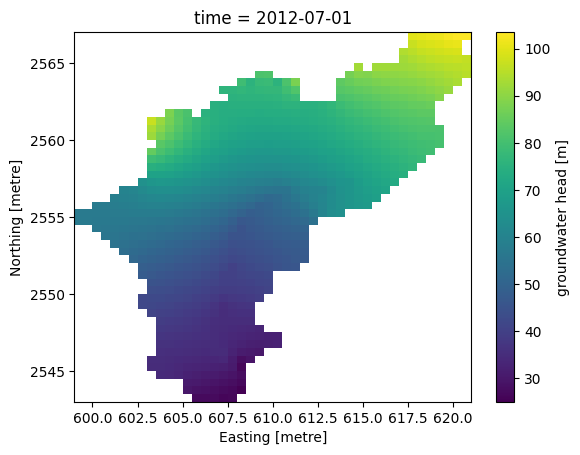
institution: BRGM, French Geological Survey, Orléans, France# on plot à un instant t
ds_3d.isel(time=-1)['charge'].plot.pcolormesh(x='x',y='y')
<matplotlib.collections.QuadMesh at 0x7700c224c620>
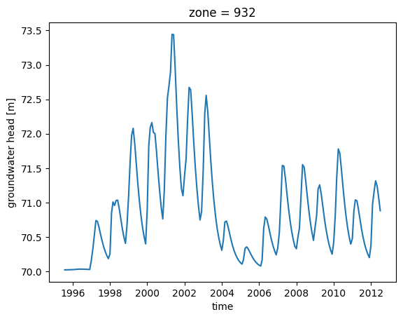
# ou la chronique dans une maille
ds.isel(zone=255)['charge'].plot()
[<matplotlib.lines.Line2D at 0x7700c21eaae0>]
Pour les gigognes, une fonction de plot spécifique est proposée (gm.plot_nested_grids()).
Pour les modèles avec plusieurs couches, on peut récupérer les couches de surfaces~: gm.get_min_layer(ds, [subset_layers=[3,5]])
ou même afficher ce résultat~: gm.plot_outcrop()
Les fonctions natives de xarray, numpy permettent d’ores-et-déjà d’accéder à certaines fonctionnalités de Operasem (substitution de valeurs, transformation, opérations entre deux grilles, etc.)
Fonctionnalités avancées
Exemple de différentes opérations entre grilles, avec xarray et gridmarthe
# compute diff between grids
ds0 = ds.sel(time='1995-11-01')
ds1 = ds.sel(time='2001-02-01')

ds0['charge'] - ds1['charge']
<xarray.DataArray 'charge' (zone: 927)> Size: 7kB
array([ 0.00000e+00,  0.00000e+00,  0.00000e+00,  0.00000e+00,
        0.00000e+00,  0.00000e+00,  0.00000e+00,  0.00000e+00,
       -3.25440e-01, -4.60980e-01, -5.27480e-01, -5.59100e-01,
       -5.74500e-01,  0.00000e+00, -3.74970e-01, -6.81720e-01,
       -8.68420e-01, -9.77570e-01, -1.04721e+00, -1.09548e+00,
        0.00000e+00, -6.41230e-01, -1.00733e+00, -1.22240e+00,
       -1.35717e+00, -1.45930e+00, -1.57370e+00, -1.80513e+00,
        0.00000e+00,  0.00000e+00,  0.00000e+00,  0.00000e+00,
       -5.66100e-01, -1.02068e+00, -1.33316e+00, -1.53087e+00,
       -1.65762e+00, -1.74995e+00, -1.82523e+00, -1.90350e+00,
        0.00000e+00,  0.00000e+00, -1.43024e+00, -1.00962e+00,
       -1.14766e+00, -8.35060e-01, -7.87260e-01, -8.78120e-01,
       -1.16742e+00, -1.45697e+00, -1.68467e+00, -1.83483e+00,
       -1.92341e+00, -1.97372e+00, -1.99069e+00, -1.98500e+00,
        0.00000e+00,  0.00000e+00, -3.44370e-01, -3.57610e-01,
        0.00000e+00,  0.00000e+00,  0.00000e+00, -2.09688e+00,
       -1.83277e+00, -1.61107e+00, -1.55613e+00, -1.44464e+00,
       -1.43203e+00, -1.52037e+00, -1.68965e+00, -1.87151e+00,
       -2.02142e+00, -2.11349e+00, -2.14897e+00, -2.14145e+00,
       -2.09989e+00, -1.43919e+00, -1.36450e+00, -9.45770e-01,
...
       -6.78740e-01, -1.82235e+00, -1.73151e+00, -1.55717e+00,
       -1.30703e+00, -9.77720e-01, -5.57570e-01, -4.35400e-02,
       -1.44860e-01, -2.52990e-01, -3.26250e-01, -3.69900e-01,
       -4.01230e-01, -5.87460e-01, -6.72990e-01, -1.76108e+00,
       -1.67109e+00, -1.50200e+00, -1.26479e+00, -9.60430e-01,
       -5.85770e-01, -1.32270e-01, -3.03400e-02, -1.52940e-01,
       -1.90000e-01, -1.65750e-01,  0.00000e+00, -1.76839e+00,
       -1.72637e+00, -1.62543e+00, -1.45758e+00, -1.23024e+00,
       -9.55270e-01, -6.37120e-01, -3.04530e-01, -2.48100e-02,
       -7.04900e-02,  0.00000e+00,  0.00000e+00, -1.75184e+00,
       -1.68804e+00, -1.58243e+00, -1.41312e+00, -1.18093e+00,
       -9.31090e-01, -6.64310e-01, -3.79320e-01, -4.50800e-02,
       -1.84200e-02, -1.20000e-02, -1.64234e+00, -1.54945e+00,
       -1.37045e+00, -1.08295e+00, -8.56250e-01, -6.43070e-01,
       -4.37550e-01, -2.51870e-01, -1.76770e-01, -1.46430e-01,
       -8.46730e-01, -6.94620e-01, -5.40770e-01, -4.04770e-01,
       -2.89830e-01, -2.15860e-01, -1.52910e-01, -6.92440e-01,
       -4.57850e-01, -3.42300e-01, -2.65000e-01, -2.01410e-01,
       -1.59930e-01,  3.00000e-05,  0.00000e+00,  0.00000e+00,
       -2.06900e-02,  0.00000e+00, -1.24820e-01])
Coordinates:
  * zone     (zone) int32 4kB 255 256 257 258 259 ... 2722 2723 2724 2725 2726
Attributes:
    varname:             CHARGE
    units:               m
    mart_missing_value:  9999.0
    standard_name:       water_table_level
long_name: groundwater head# compute quantile
ds_5perc = ds.copy()
ds_5perc['q5'] = ds_5perc['charge'].quantile(0.05, dim='time')
ds_5perc['tresh'] = ds_5perc['charge'] < ds_5perc['q5']
ds_5perc
<xarray.Dataset> Size: 2MB
Dimensions:   (time: 205, zone: 927)
Coordinates:
  * time      (time) datetime64[ns] 2kB 1995-07-31 1995-08-01 ... 2012-07-01
  * zone      (zone) int32 4kB 255 256 257 258 259 ... 2722 2723 2724 2725 2726
    quantile  float64 8B 0.05
Data variables:
    charge    (time, zone) float64 2MB 100.0 100.6 101.1 ... 27.0 26.0 26.35
    x         (zone) float32 4kB 617.8 618.2 618.8 619.2 ... 606.8 607.2 607.8
    y         (zone) float32 4kB 2.567e+03 2.567e+03 ... 2.543e+03 2.543e+03
    dx        (zone) float32 4kB 0.5 0.5 0.5 0.5 0.5 0.5 ... 0.5 0.5 0.5 0.5 0.5
    dy        (zone) float32 4kB 0.5 0.5 0.5 0.5 0.5 0.5 ... 0.5 0.5 0.5 0.5 0.5
    izone     (zone) int32 4kB 1 2 3 4 5 6 7 8 ... 921 922 923 924 925 926 927
    q5        (zone) float64 7kB 100.0 100.6 101.1 101.6 ... 26.98 26.0 26.31
    tresh     (time, zone) bool 190kB False False False ... False False False
Attributes: (12/17)
    conventions:          CF-1.10
    title:                Modélisation du bassin de la SOMME Nappe_Libre
    marthe_grid_version:  9.0
    original_dimensions:  x,y,z [grids]: 53 54 1
    crs:                  {'crs_wkt': 'PROJCRS["NTF (Paris) / Lambert zone II...
    lon_resolution:       0.5
    ...                   ...
    period:               1995-2012
    frequency:            30 day(s)
    creation_date:        Created on 2026-05-27T07:31:59Z UTC
    comment:              Hydrogeological model created with MARTHE code (Thi...
    domain:               FR-France
institution: BRGM, French Geological Survey, Orléans, France# compute anomaly
anom = ds.groupby("time.month") - ds.groupby("time.month").median(dim="time")
# rename new variable
ds_anom = ds.copy()
ds_anom['anom'] = anom['charge']
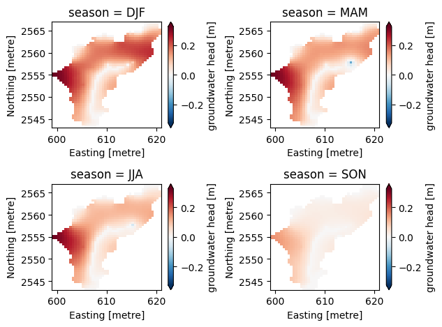
# compute seasonal mean
# 1st: mean head over each season...
ds_season = ds_anom.resample(time="QS-DEC").median(dim='time') # or .agg({"time": 'mean'})
# ... then aggregate all seasons
ds_season_agg = ds_season.groupby("time.season").mean(dim="time")
ds_season_agg  # mind the new dimension 'season'
<xarray.Dataset> Size: 152kB
Dimensions:  (season: 4, zone: 927)
Coordinates:
  * season   (season) object 32B 'DJF' 'JJA' 'MAM' 'SON'
  * zone     (zone) int32 4kB 255 256 257 258 259 ... 2722 2723 2724 2725 2726
Data variables:
    charge   (season, zone) float64 30kB 100.0 100.6 101.1 ... 26.99 26.0 26.33
    x        (season, zone) float32 15kB 617.8 618.2 618.8 ... 606.8 607.2 607.8
    y        (season, zone) float32 15kB 2.567e+03 2.567e+03 ... 2.543e+03
    dx       (season, zone) float32 15kB 0.5 0.5 0.5 0.5 0.5 ... 0.5 0.5 0.5 0.5
    dy       (season, zone) float32 15kB 0.5 0.5 0.5 0.5 0.5 ... 0.5 0.5 0.5 0.5
    izone    (season, zone) float64 30kB 1.0 2.0 3.0 4.0 ... 925.0 926.0 927.0
    anom     (season, zone) float64 30kB 0.0 0.0 0.0 ... -0.002924 0.0 0.001059
Attributes: (12/17)
    conventions:          CF-1.10
    title:                Modélisation du bassin de la SOMME Nappe_Libre
    marthe_grid_version:  9.0
    original_dimensions:  x,y,z [grids]: 53 54 1
    crs:                  {'crs_wkt': 'PROJCRS["NTF (Paris) / Lambert zone II...
    lon_resolution:       0.5
    ...                   ...
    period:               1995-2012
    frequency:            30 day(s)
    creation_date:        Created on 2026-05-27T07:31:59Z UTC
    comment:              Hydrogeological model created with MARTHE code (Thi...
    domain:               FR-France
institution: BRGM, French Geological Survey, Orléans, France# set coords for plot
ds_season_agg.update({
v: ds_season_agg[v].isel(season=0) # remove season dim for coordinates, appears in computation
for v in ['x', 'y', 'dx', 'dy']
})
ds_season_agg_2d = gm.assign_coords(ds_season_agg)
# Seasonal plot
import numpy as np
from matplotlib import pyplot as plt, colors

var = 'anom'
minval, maxval = ds_season_agg_2d[var].min(skipna=True).values, ds_season_agg_2d[var].max(skipna=True).values
fig, axes = plt.subplots(nrows=2, ncols=2)
axes = axes.ravel()
for i, season in enumerate(("DJF", "MAM", "JJA", "SON")):
    ds_season_agg_2d[var].sel(season=season).plot.pcolormesh(
            # x="x", y="lat",
            ax=axes[i],
            # cmap="Spectral",
            # vmin=minval, vmax=maxval,
            norm=colors.CenteredNorm(halfrange=np.max(np.abs([minval, maxval]))),
            add_colorbar=True,
            extend="both",
        )
plt.tight_layout()